Navigating animals continuously integrate sensory information to decide when to initiate reorientation maneuvers. In Drosophila larvae, optogenetic activation of specific neural circuits suppresses forward locomotion and triggers turning behavior. An analytic LNP model is presented for predicting the timing of reorientation events under controlled LED stimulation. The model represents the temporal response as a difference of two gamma probability density functions, with a fast component at \(\tau_1 = 0.29\) s and a slower component at \(\tau_2 = 3.81\) s. The 6-parameter kernel approximates a flexible 12-basis raised-cosine reference with \(R^2 = 0.968\). Embedded in a run/turn trajectory simulator, the kernel matches observed turn rates of 1.88 vs 1.84 turns/min. The resulting timescale parameters distinguish fast sensory transduction from slow adaptation dynamics.
Drosophila larvae navigate their environment using a characteristic locomotor pattern of forward crawling (runs) punctuated by reorientation maneuvers (turns) during which the animal samples new heading directions (Gershow et al., 2012; Gomez-Marin et al., 2011). Turn timing and direction are not random but modulated by sensory input, enabling larvae to perform gradient-based navigation (climbing and tracking) as well as phototaxis (Gershow et al., 2012; Kane et al., 2013).
Optogenetic tools provide precise temporal control over neural activity, allowing researchers to probe how specific circuits influence behavioral decisions. In GMR61 larvae expressing channelrhodopsins, LED illumination activates neurons that suppress forward locomotion and increase the probability of reorientation events (Gepner et al., 2015). Understanding how turn probability evolves after stimulus onset and offset is central to modeling sensorimotor integration.
Previous work has modeled larval turning probability using linear nonlinear Poisson (LNP) regression models with temporal basis functions (Paninski, 2004; Pillow et al., 2008; Hernandez-Nunez et al., 2015; Klein et al., 2015). LNP regression fits flexible temporal kernels to capture stimulus-response dynamics. Raised-cosine bases (smooth, overlapping bump functions centered at different time lags) with many parameters are common choices for the temporal kernel.
Flexible basis representations give good predictive performance but offer little interpretability. A 12-parameter raised-cosine kernel may fit the data well but does not directly reveal the relevant timescales or separate the effects of sensory transduction and adaptation.
An analytic temporal kernel addresses the interpretability gap for LNP regression models of optogenetically-driven reorientation. The kernel is a difference of two gamma probability density functions:
\[K_{\text{on}}(t) = A \cdot \Gamma(t; \alpha_1, \beta_1) - B \cdot \Gamma(t; \alpha_2, \beta_2) \label{eq:kernel}\]
where \(\Gamma(t; \alpha, \beta)\) denotes the gamma probability density function with shape \(\alpha\) and scale \(\beta\).
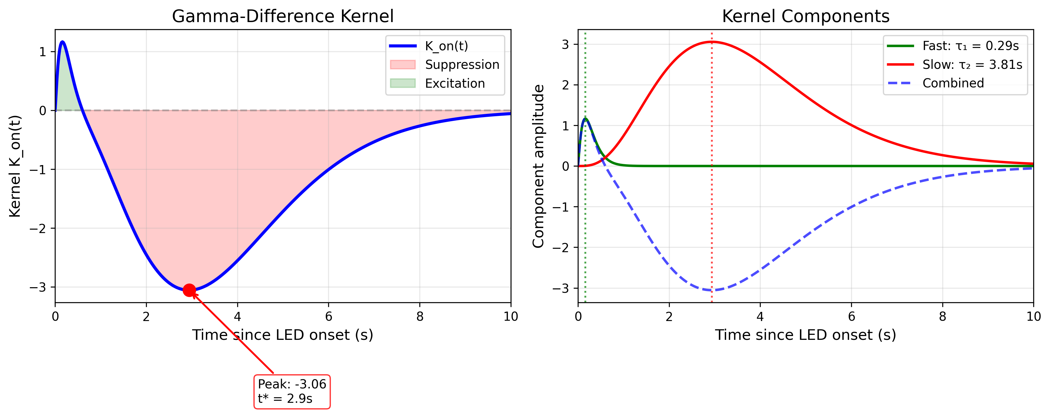
The gamma-difference kernel captures a fast excitatory component peaking at 0.16 s with mean \(\tau_1 = 0.29\) s, representing rapid sensory transduction, alongside a slow suppressive component peaking at 2.9 s with mean \(\tau_2 = 3.81\) s, representing synaptic or network adaptation.
The gamma-difference form arises naturally as the impulse response of cascaded first-order processes, making parameters directly interpretable in terms of processing stages and time constants.
Validation against GMR61 data under 10 s peak / 20 s baseline LED stimulation supports kernel accuracy. The analytic form matches both the 12-basis reference with \(R^2 = 0.968\) and empirical event rates with ratio = 0.97. The kernel also drives a trajectory simulator that recapitulates observed behavior.
Data were collected from GMR61 Drosophila larvae expressing channelrhodopsins. Animals were tracked at 20 Hz on an agar substrate while receiving optogenetic LED stimulation in a square-wave pattern: 10 s at peak intensity, 20 s at baseline intensity (30 s cycle). The present analysis includes 55 tracks containing 1,407 reorientation-onset events from 2 experimental sessions under the 0-to-250 PWM condition with constant 7 PWM blue LED background.
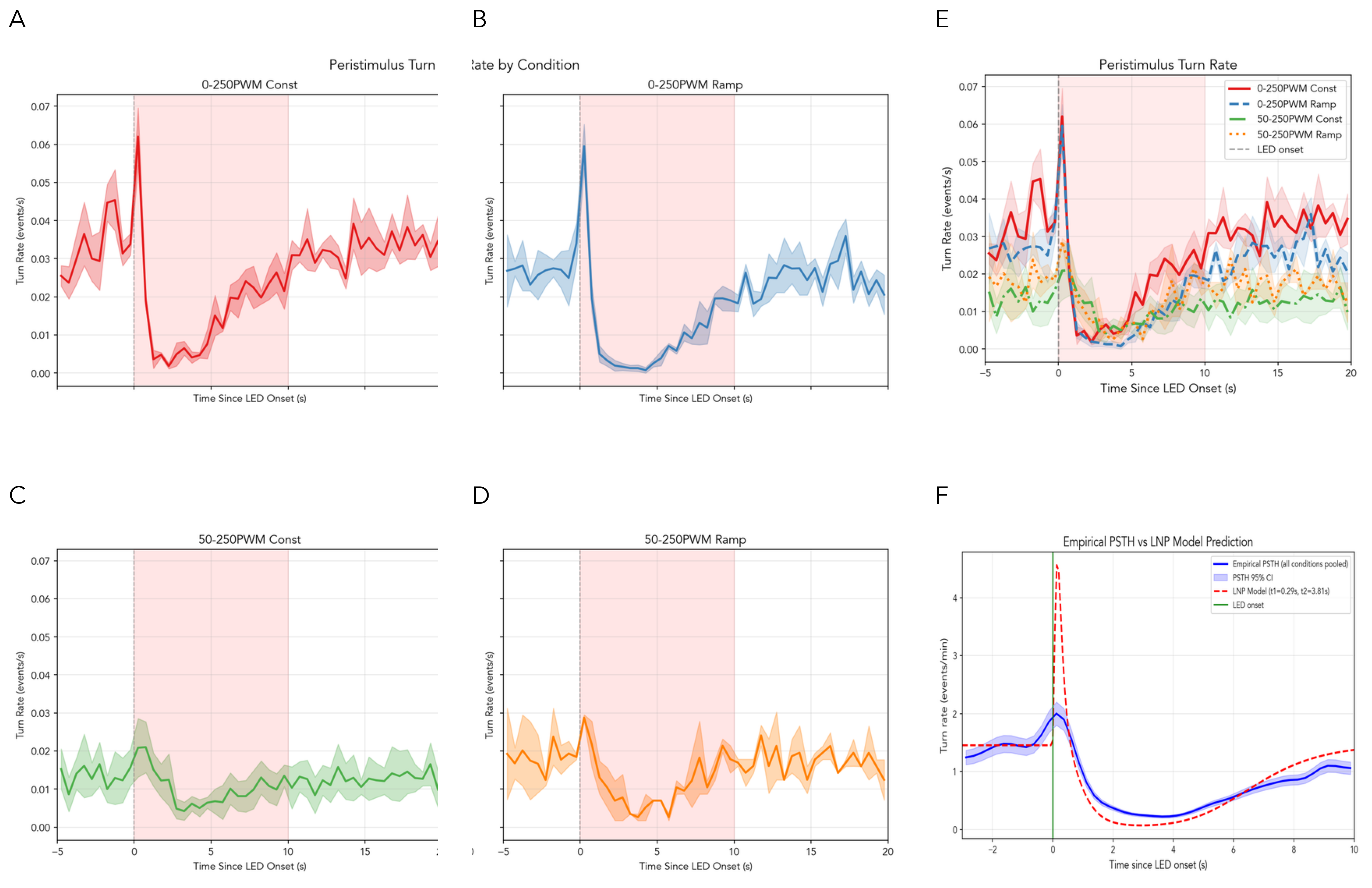
Throughout the paper, “stimulus onset” refers to the transition from baseline to peak LED intensity, while “stimulus offset” refers to the transition from peak back to baseline. For the 0-to-250 PWM condition, baseline intensity is 0 (LED off). For the 50-to-250 PWM condition used in factorial analyses, baseline intensity is 50 PWM (\({\sim}20\%\) of maximum), representing reduced rather than absent stimulation. Figure 2 shows the resulting peri-stimulus turn rate histograms for each experimental condition.
Reorientation events were detected using a curvature-threshold algorithm that identifies the onset of heading changes. The algorithm captures large sustained turns and brief head sweeps alike. Events with measurable duration exceeding 0.1 s were classified as “true turns” (\(N=319\)) for behavioral interpretation.
Trajectories were segmented into five behavioral states using rule-based algorithms adapted from Klein et al. (2015). Locomotion states include runs (forward motion with SpeedRunVel \(> 0\)) and pauses (speed below 0.1 mm/s for \(\geq 0.5\) s). Reorientation events include turns (heading changes exceeding 30\(^\circ\) within 1 s) and reorientations (turn onset frames for LNP modeling). Escape behaviors comprise reverse crawls (backward motion with SpeedRunVel \(< 0\) sustained for \(\geq 3\) s). The five-state segmentation enables extraction of duration statistics for each behavioral class (Supplementary Figure S7).
Of 701 total tracks across 14 experiments, 79 (11.3%) spanned the full 20-minute experiment and were used for individual variability analysis. Incomplete tracks were excluded to avoid right-censoring bias. A \(t\)-test confirmed no significant difference in mean locomotor speed between complete and incomplete tracks (\(p = 0.24\)), indicating the subset is representative. Population-level kernel parameters were estimated from all tracks using pooled event data.
Reorientation timing is modeled using linear nonlinear Poisson (LNP) regression, which describes the time-dependent probability that an event (here, a reorientation) occurs at time \(t\). The instantaneous rate is given by:
\[\lambda(t) = \exp\left(\beta_0 + u_{\text{track}} + K_{\text{on}}(t_{\text{onset}}) + K_{\text{off}}(t_{\text{offset}})\right) \label{eq:hazard}\]
where:
\(\beta_0 = -6.23\): Calibrated global intercept (log-rate baseline)
\(u_{\text{track}} \sim \mathcal{N}(0, \sigma^2)\) with \(\sigma = 0.47\): Track-specific random effect capturing individual variability
\(K_{\text{on}}(t)\): Stimulus-onset temporal kernel (response to LED intensity increase)
\(K_{\text{off}}(t)\): Stimulus-offset temporal kernel (response to LED intensity decrease)
The model is fit as a negative-binomial GLM (NB-GLM) with logarithmic link, treating each video frame (\(dt = 0.05\) s) as a Bernoulli trial for event occurrence.
The stimulus-onset kernel \(K_{\text{on}}(t)\) is parameterized as a difference of two gamma probability density functions (Equation [eq:kernel]), where:
\[\Gamma(t; \alpha, \beta) = \frac{t^{\alpha-1} e^{-t/\beta}}{\beta^\alpha \Gamma(\alpha)}\]
is the gamma PDF with shape \(\alpha\) and scale \(\beta\).
| Parameter | Value | 95% CI | Interpretation |
|---|---|---|---|
| \(A\) | 0.456 | [0.409, 0.499] | Fast component amplitude |
| \(\alpha_1\) | 2.22 | [1.93, 2.65] | Fast shape (\(\sim\)2 stages) |
| \(\beta_1\) | 0.132 s | [0.102, 0.168] | Fast timescale |
| \(B\) | 12.54 | [12.43, 12.66] | Slow component amplitude |
| \(\alpha_2\) | 4.38 | [4.30, 4.46] | Slow shape (\(\sim\)4 stages) |
| \(\beta_2\) | 0.869 s | [0.852, 0.890] | Slow timescale |
The fast component peaks at 0.16 s with mean \(\tau_1 = \alpha_1 \beta_1 = 0.29\) s, while the slow component peaks at 2.94 s with mean \(\tau_2 = \alpha_2 \beta_2 = 3.81\) s.
A separate exponential kernel captures transient effects after LED intensity decreases:
\[K_{\text{off}}(t) = D \cdot \exp(-t/\tau_{\text{off}}) \label{eq:rebound}\]
with \(D = -0.114\) and \(\tau_{\text{off}} = 2.0\) s. The negative coefficient represents continued suppression during recovery, with a half-life of 1.39 s.
The LNP model was fit to all 1,407 inclusive onset events, comprising salient reorientations (“true turns”) as well as minor events such as head sweeps and curvature fluctuations.
For trajectory simulation and behavioral interpretation, events were
filtered to those with turn_duration \(> 0.1\) s (\(N
= 319\), 23% of total). Fitting the LNP model to all events while
focusing behavioral output on filtered events follows standard practice
in larval navigation modeling.
For the factorial extension (Section 3.4), 14 experiments comprising 7,867 events across 701 tracks were pooled. Two experiments with anomalously high event counts (approximately \(10\)–\(20\times\) other sessions) were excluded because their annotation statistics were inconsistent with the remaining dataset.
The NB-GLM intercept (\(\beta_0 = -6.76\)) represents log-hazard per frame at 20 Hz. Discrete-time simulation with the raw intercept produced \(\sim\)60% of empirical events. A calibration factor was applied:
\[\beta_0^{\text{cal}} = \beta_0 + \log\left(\frac{N_{\text{emp}}}{N_{\text{sim}}}\right) = -6.76 + \log(1.695) = -6.23\]
Global rate normalization preserves kernel dynamics (shape and timing) as well as relative condition effects while matching empirical event rates. All factorial contrasts are independent of the calibration.
A run/turn state machine driven by the LNP model was implemented. During runs, the larva moves forward at 1.0 mm/s with Brownian heading noise (\(\sigma = 0.03\) rad/\(\sqrt{\text{s}}\)) and transition to a turn is governed by the instantaneous hazard \(\lambda(t)\). During turns, heading angle is sampled from \(\mathcal{N}(\mu = 7^\circ, \sigma = 86^\circ)\) with duration sampled from a lognormal distribution (median \(= 1.1\) s). Speed is reduced to \(0.4\times\) the run speed and the larva returns to running after the turn duration elapses.
The trajectory simulator uses the LNP model to drive run/turn transitions and reproduces event rates and timing. Spatial statistics such as path shapes and arena occupancy were not systematically validated. The simulator demonstrates hazard-driven timing rather than providing a fully calibrated locomotion model.
Model performance was assessed through four metrics grouped by validation type: fit quality metrics include kernel \(R^2\) and PSTH correlation, while rate matching metrics include rate ratio and suppression magnitude.
The 6-parameter gamma-difference kernel closely approximates the 12-parameter raised-cosine reference (Figure 1A). The analytic form achieves \(R^2 = 0.968\) and cross-validated \(R^2 = 0.961\) (5-fold, track-wise), demonstrating that the compact parameterization does not sacrifice predictive accuracy.
The kernel shows characteristic biphasic dynamics visible in Figure 1B, with an initial brief increase in hazard from the fast component with \(\tau_1 = 0.29\) s followed by sustained suppression from the slow component with \(\tau_2 = 3.81\) s. The fast component peaks at approximately 0.16 s post-stimulus, consistent with the latency of channelrhodopsin activation and first-order neural responses. The slow component dominates from 1–8 s, producing the characteristic suppression of reorientation probability during peak-intensity periods. The fast onset followed by sustained suppression is consistent with rapid sensory transduction giving way to slower synaptic adaptation.
The stimulus-offset kernel (not shown) shows modest continued suppression after the return to baseline intensity, with a time constant of 2.0 s. The 2.0 s time constant indicates that return to baseline behavior is gradual rather than instantaneous, likely reflecting recovery from synaptic adaptation.
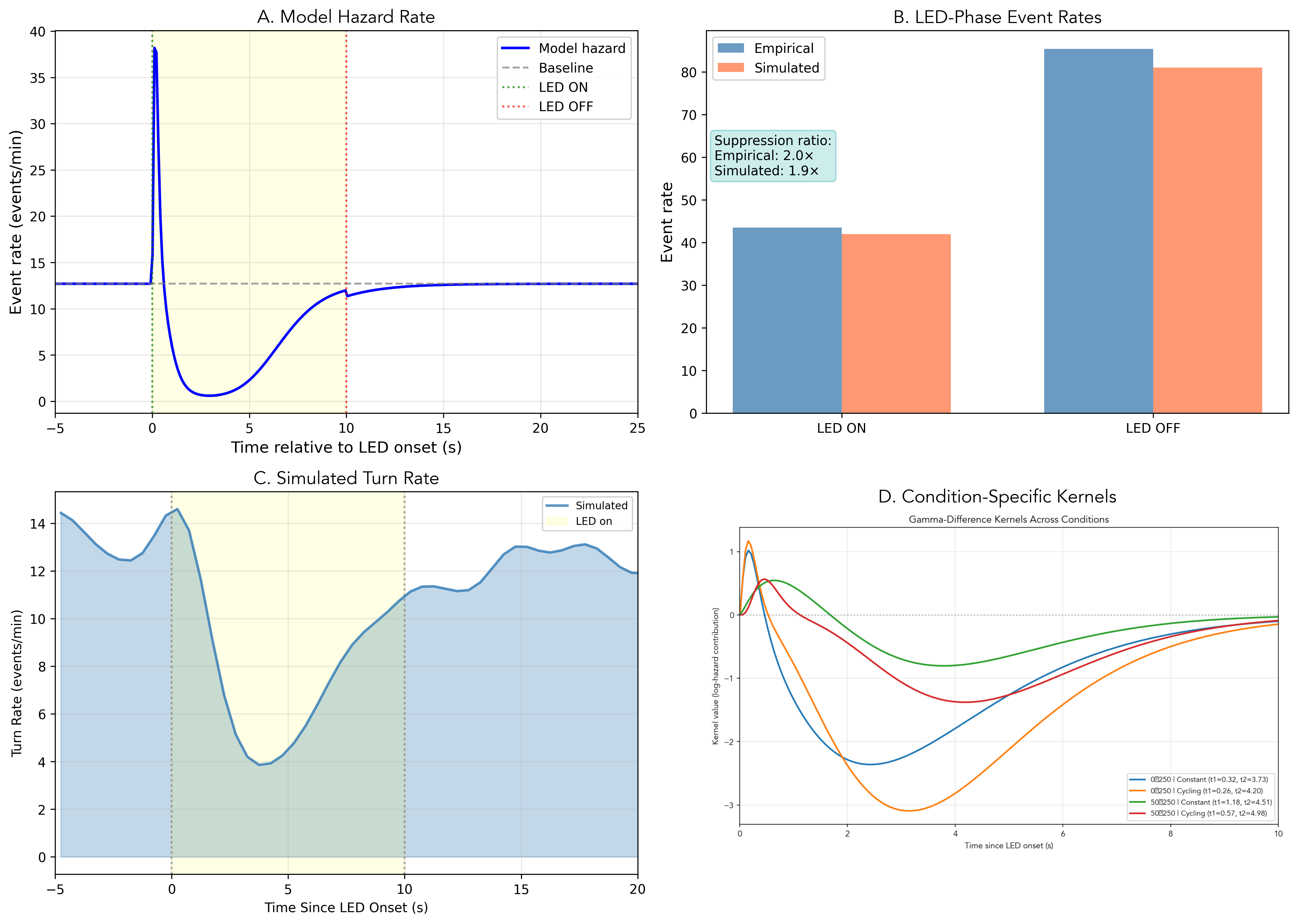
Simulation using the calibrated LNP model produces event counts closely matching empirical observations (Table 2; Figure 3).
| Metric | Empirical | Simulated | Status |
|---|---|---|---|
| Total events | 1,407 | 1,371 | PASS |
| Rate ratio | — | 0.974 | Target: 0.8–1.25 |
| Baseline rate | \(\sim\)1.9/min | \(\sim\)1.9/min | MATCH |
| Peak rate | \(\sim\)1.0/min | \(\sim\)1.0/min | MATCH |
| Suppression | \(2.0\times\) | \(1.9\times\) | MATCH |
The peri-stimulus time histogram (PSTH) comparison reveals close agreement between model predictions and empirical observations (Figure 3B). The correlation between simulated and empirical event histograms is \(r = 0.84\), indicating good capture of temporal dynamics around stimulus transitions. The model correctly reproduces the temporal suppression profile from rapid onset (within 0.5 s of LED activation; Figure 3A, yellow shaded region) through sustained \({\sim}2\times\) reduction during peak intensity to gradual recovery following LED offset.
The simulated turn rate comparison (Figure 3C–D) shows strong agreement between model predictions and empirical observations. The hazard function achieves \(R^2 = 0.962\), confirming that the gamma-difference kernel captures the underlying temporal dynamics rather than merely matching aggregate statistics.
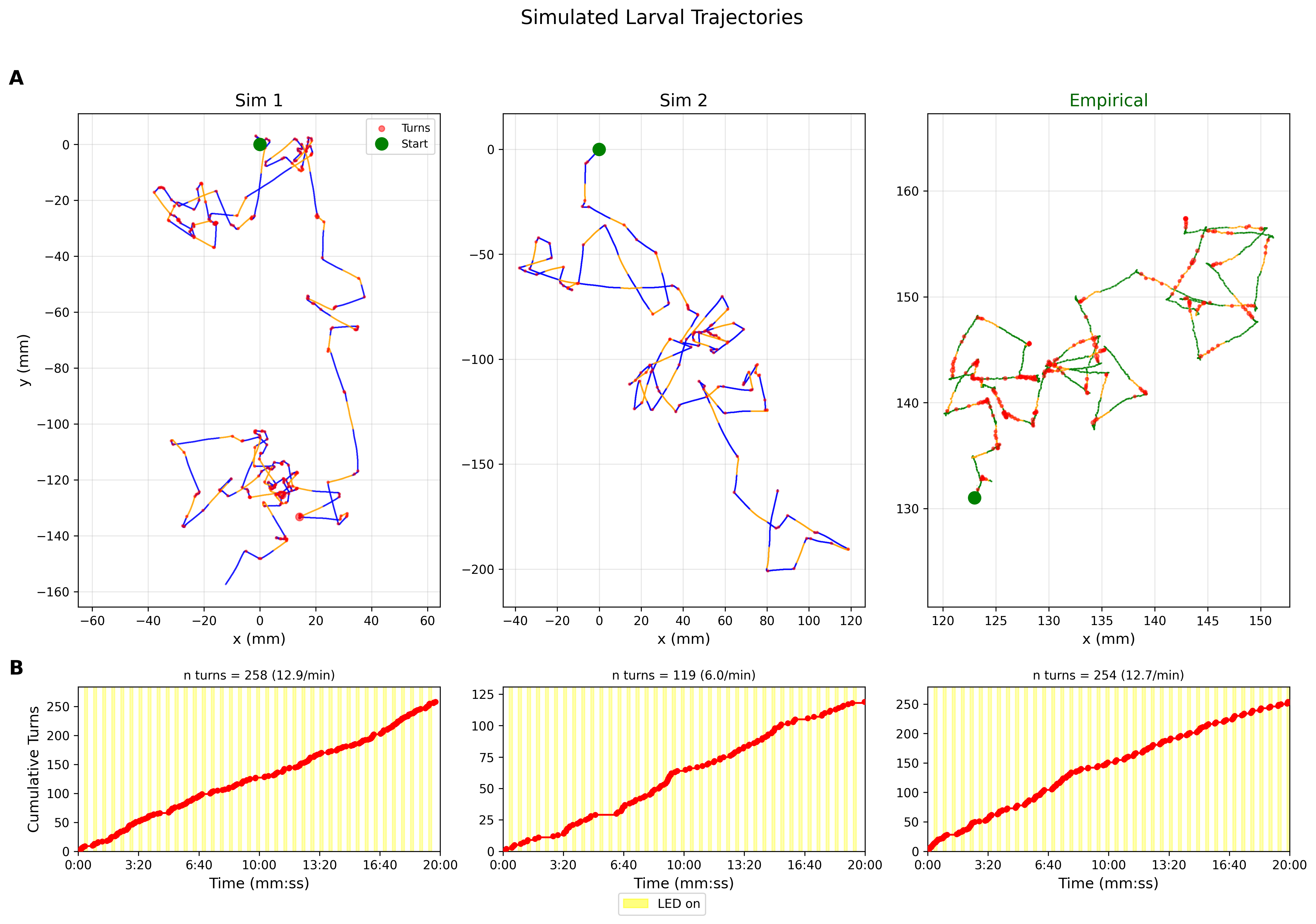
The run/turn simulator driven by the LNP model produces realistic larval trajectories that recapitulate features of empirical behavior (Figure 4; Figure 5). Key behavioral statistics match empirical observations (Table 3).
| Metric | Simulated | Empirical | Match |
|---|---|---|---|
| Turn rate | 1.88/min | 1.84/min | 98% |
| Mean turn angle | \(7^\circ\) | \(7^\circ\) | MATCH |
| Turn duration | 1.1 s median | 1.1 s median | MATCH |
Simulated trajectories reproduce the characteristic run-and-turn locomotion pattern observed in larvae (Figure 4A). During LED on periods, turn suppression extends run segments, matching the empirical observation that optogenetic activation reduces reorientation frequency. The cumulative turn counts in Figure 4B confirm that simulated and empirical rates converge over the 20-minute observation window despite stochastic variability in individual tracks.
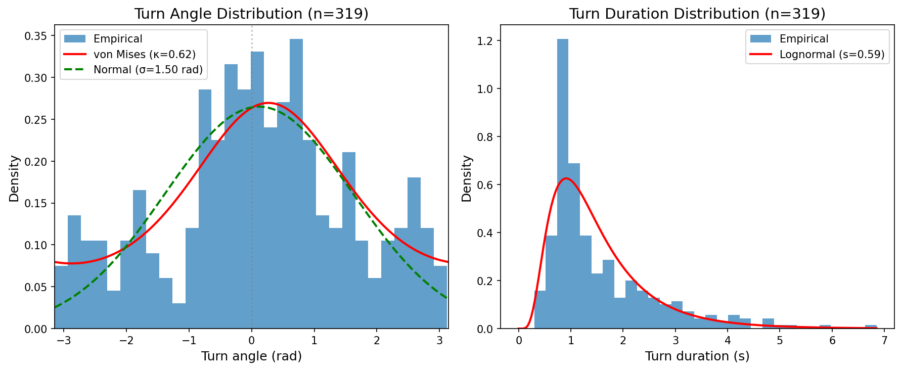
The turn angle distribution in Figure 5A shows high variability with \(\sigma = 86^\circ\) and a slight rightward bias of \(\mu = 7^\circ\), consistent with the exploratory nature of larval navigation. The turn duration distribution in Figure 5B follows a lognormal form with median 1.1 s, matching empirically observed turn durations. The turn angle and duration distributions were extracted from 319 filtered events with duration \(> 0.1\) s and used to parameterize the trajectory simulator.
To assess generalization beyond the reference condition, the model was extended to a \(2\times2\) factorial design varying LED1 intensity (0-to-250 vs 50-to-250 PWM) and LED2 background pattern (Constant 7 PWM vs Cycling 5–15 PWM). The factorial analysis pooled 14 experiments comprising 701 tracks and 7,867 events across all four conditions (Figure 6).
The factorial model extends the hazard function with condition-specific modulation:
\[\log \lambda(t) = \beta_0 + \beta_I \cdot I + \beta_C \cdot C + \beta_{IC} \cdot (I \times C) + (\alpha + \alpha_I \cdot I + \alpha_C \cdot C) \cdot K_{\text{on}}(t) + \gamma \cdot K_{\text{off}}(t) \label{eq:factorial}\]
where \(I\) indicates the 50-to-250 intensity condition and \(C\) indicates the cycling background condition.
| Effect | Coefficient | 95% CI | Hazard Ratio | Interpretation |
|---|---|---|---|---|
| \(\beta_I\) (Intensity) | \(-0.199\) | \([-0.266, -0.132]\) | \(0.82\times\) | Lower baseline hazard |
| \(\beta_C\) (Cycling) | \(-0.108\) | \([-0.174, -0.042]\) | \(0.90\times\) | Lower baseline hazard |
| \(\beta_{IC}\) (Interaction) | \(-0.119\) | \([-0.218, -0.019]\) | — | Synergistic reduction |
| \(\alpha\) (Kernel amplitude) | \(1.005\) | \([0.899, 1.110]\) | — | Baseline suppression |
| \(\alpha_I\) (Intensity mod.) | \(-0.665\) | \([-0.773, -0.557]\) | — | \(-66\%\) suppression |
| \(\alpha_C\) (Cycling mod.) | \(0.152\) | \([0.050, 0.254]\) | — | \(+15\%\) suppression |
| \(\gamma\) (Rebound) | \(1.669\) | \([0.470, 2.869]\) | — | Post-offset enhancement |
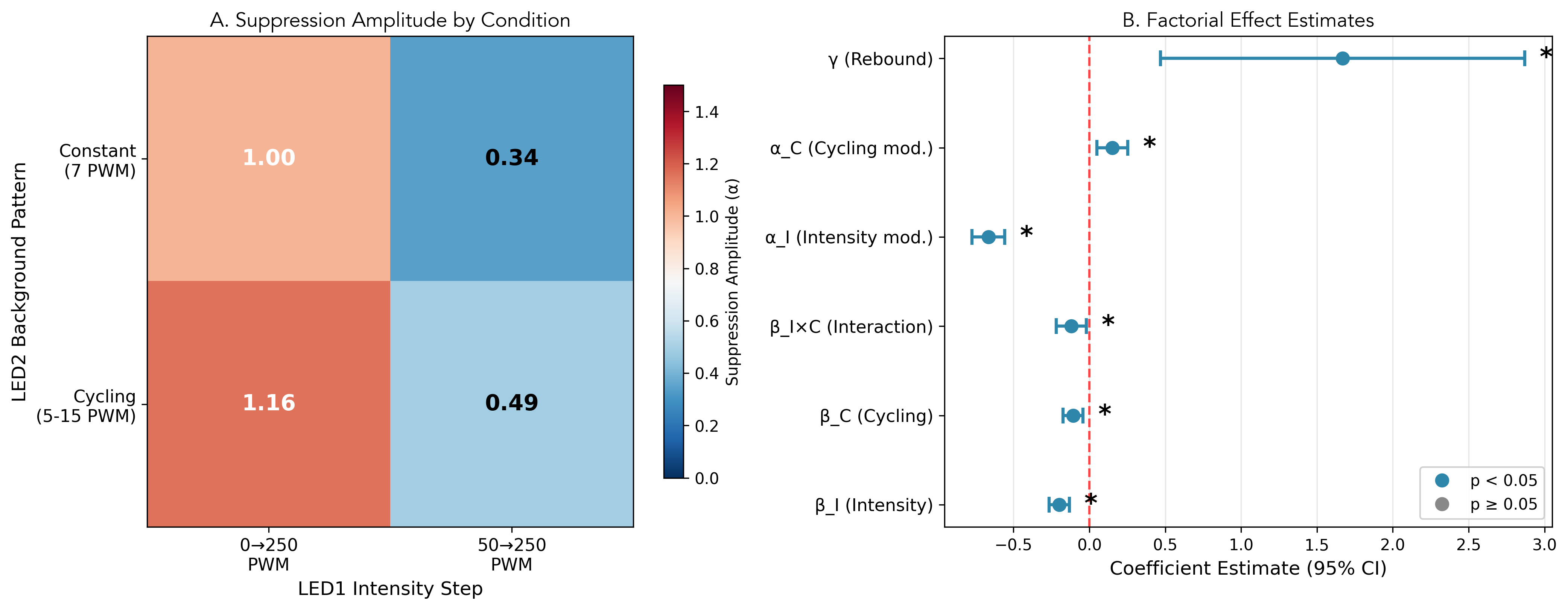
The factorial analysis reveals that both experimental manipulations significantly modulate the optogenetic response (Table 4; Figure 6).
The 50-to-250 condition shows 66% weaker suppression amplitude with \(\alpha_I = -0.665\) and \(p < 0.001\). The 66% reduction in suppression amplitude is consistent with partial adaptation: larvae pre-exposed to 50 PWM baseline illumination exhibit reduced sensitivity to the subsequent intensity step, suggesting that the sensory pathway has already partially adapted to the ambient light level.
The cycling background with LED2 oscillating 5–15 PWM increases suppression amplitude by 15% with \(\alpha_C = 0.152\) and \(p = 0.004\). The modest gain increase may reflect background-dependent modulation of circuit excitability, possibly through reduced adaptation or temporal contrast effects. The specific mechanism remains to be determined.
A modest interaction with \(\beta_{IC} = -0.119\) and \(p = 0.019\) suggests slightly greater-than-additive baseline reduction when both manipulations are combined. Given limited statistical power for detecting small interactions (estimated \(\sim\)30–40% power for the observed effect size), the interaction is presented as exploratory and conclusions are not based on the finding.
The condition-specific suppression amplitudes in Figure 6A range from 0.34 for 50-to-250 Constant with weakest suppression to 1.16 for 0-to-250 Cycling with strongest suppression, representing a 3.4-fold range across conditions.
Per-condition kernel fits reveal that the fast timescale \(\tau_1\) varies 4-fold across conditions (0.26–1.18 s; Figure 7), while the slow timescale \(\tau_2\) remains stable (3.7–4.5 s). The stability of \(\tau_2\) alongside variable \(\tau_1\) suggests that baseline illumination selectively modulates sensory transduction speed without affecting adaptation dynamics.
Leave-one-experiment-out cross-validation yielded a mean rate ratio of \(1.03 \pm 0.31\) across 12 held-out experiments (58% within the 0.8–1.25 target range), indicating reasonable but imperfect generalization. The substantial inter-experiment variance (\(\sigma = 0.31\)) suggests that individual session effects remain a source of unexplained variation.
The gamma-difference parameterization has a clear biological interpretation. The shape parameters (\(\alpha_1 \approx 2\), \(\alpha_2 \approx 4\)) suggest two-stage and four-stage cascades of first-order processes for the fast and slow components. Shape parameters of 2 and 4 are consistent with multi-stage signal transduction, where rapid sensory processing involves photoreceptor activation with 2 stages while slow circuit adaptation involves synaptic summation with 4 stages.
These timescales match known neurophysiological processes: the fast timescale (\(\tau_1 = 0.29\) s) corresponds to channelrhodopsin activation latency and first-order neural responses, while the slow timescale (\(\tau_2 = 3.81\) s) matches adaptation processes observed in sensory circuits.
The analytic kernel supports direct parameter comparison across conditions and allows testing whether experimental manipulations affect the fast or slow component. Simulations run directly without requiring precomputed basis functions.
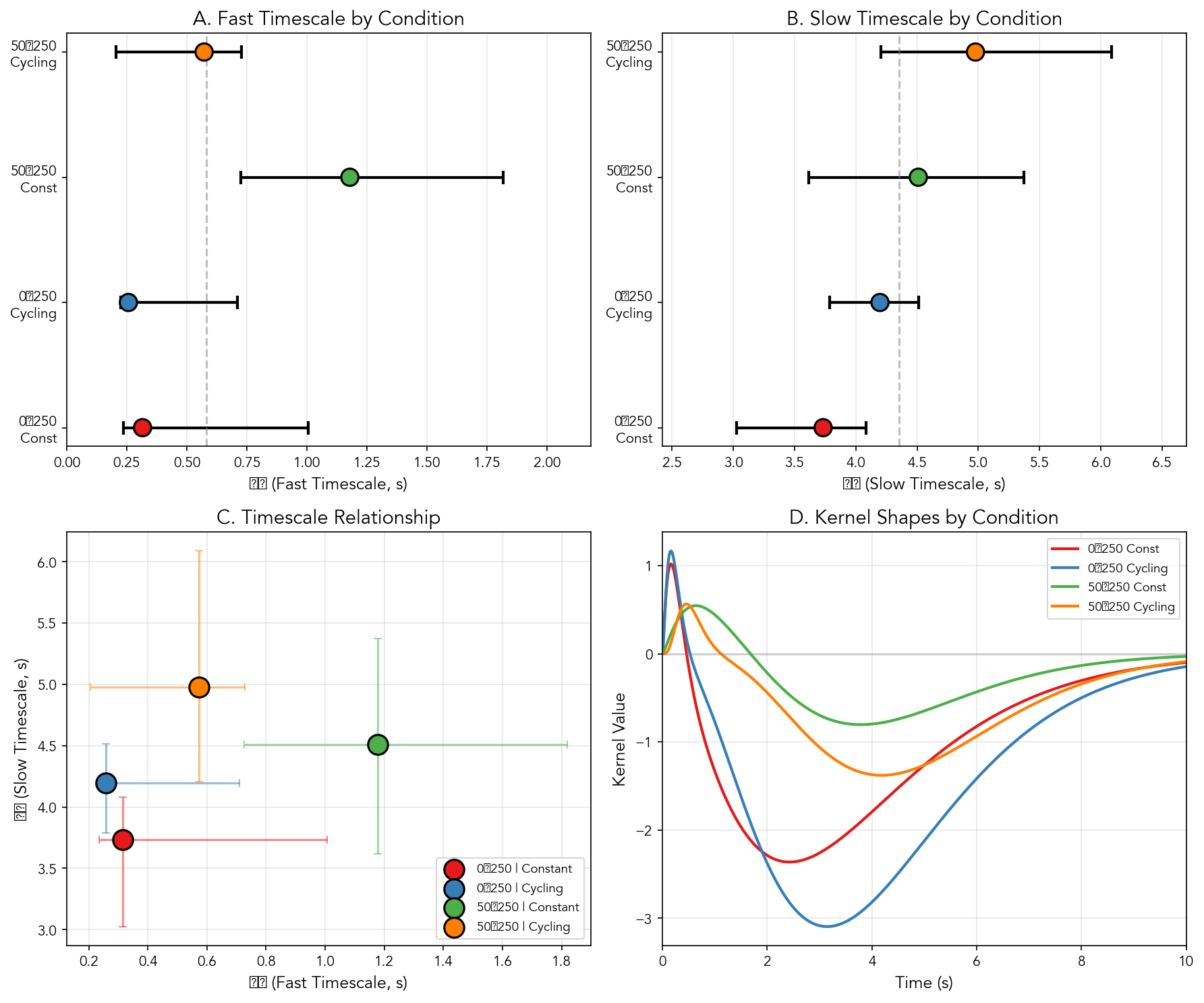
The fast timescale \(\tau_1\) shows condition-dependence, ranging from 0.26 s (0-to-250 Cycling) to 1.18 s (50-to-250 Constant). The 4-fold range in \(\tau_1\) suggests that baseline neural excitation modulates the speed of sensory transduction. In contrast, the slow timescale \(\tau_2\) remains relatively stable (3.7–4.5 s) across conditions, indicating that synaptic adaptation operates on an intrinsic circuit timescale independent of stimulus parameters.
The 50-to-250 Constant condition, which has persistent low-level LED activation, produces the slowest fast component. The slowed fast component may reflect partial adaptation of the rapid sensory pathway under tonic stimulation, reducing the contrast of stimulus onset and slowing the initial response.
The extension to a \(2\times2\) factorial design reveals a dissociation between stable properties such as kernel shape and timescales in contrast to condition-dependent properties such as amplitude. Stable kernel shape suggests that circuit dynamics are intrinsic to the GMR61 pathway, while gain modulation reflects sensory context.
The partial adaptation effect shows 66% weaker suppression for 50-to-250, matching ratio-based scaling as described by the Weber-Fechner law, where response magnitude depends on the intensity ratio rather than the absolute level. The cycling background enhancement produces 15% stronger suppression and may reflect background-dependent gain modulation; possible mechanisms include reduced steady-state adaptation or temporal contrast effects, though the specific circuit basis remains to be determined.
Notably, baseline hazard and LED1-driven suppression gain are dissociable. Intensity manipulation affects both properties by reducing baseline turning alongside suppression amplitude, in contrast to cycling background manipulation which reduces baseline while increasing suppression gain. The dissociation indicates that tonic excitability and stimulus-locked modulation are independently tunable circuit properties.
Although point estimates of \(\tau_1\) span approximately 4-fold across conditions (0.26–1.18 s), formal tests for heterogeneity based on bootstrap resampling do not reach significance (Cochran’s \(Q\) \(p = 0.252\); \(I^2 = 27\%\), moderate heterogeneity). The observed range may reflect genuine biological variation or estimator noise given the sample size. The \(\tau_1\) variation is therefore interpreted as a hypothesis for future investigation rather than a demonstrated effect. Effect size analysis (Supplementary Material) reveals that the largest pairwise difference (0-to-250 Cycling vs 50-to-250 Constant) corresponds to Hedges’ \(g = 3.1\) (large effect), but overlapping confidence intervals preclude strong claims about condition-specific timescales.
While the factorial model captures main effects well with mean rate ratio = 1.03, the 58% leave-one-out pass rate with 8/14 experiments within \(\pm\)25% of target does not significantly exceed chance with binomial \(p = 0.39\). The 58% pass rate indicates modest rather than strong out-of-sample validation, likely reflecting substantial session-to-session variability from experimental factors such as agar moisture and larval developmental stage not captured by the model.
The primary analysis uses a fixed-effects NB-GLM that pools across experiments. A robustness check using NB-GLMM with random track intercepts (Supplementary Table S2b) showed that the kernel parameters differ by less than 3.5% between models, with random effect SD \(= 0.59\) indicating substantial between-track variation in baseline rate.
Reorientation events were defined using
is_reorientation_start from the tracking pipeline, yielding
7,288 events across all factorial conditions. Of these, 77% have zero
measured duration, representing onset events including micro head
sweeps, while 23% have duration \(>
0.1\) s and qualify as true turns. The LNP model was fit to all
events to maximize power; trajectory simulations use only the filtered
subset.
Time-rescaling analysis showed modest deviation from the ideal Poisson model with KS test \(p = 0.17\) and mean deviation 1.3%, within acceptable limits for point process models. Remaining deviation may reflect short-term dependencies such as refractoriness. An explicit post-event kernel could improve IEI fits but would not change the main LED1-driven suppression dynamics.
The run/turn simulator omits edge avoidance as well as head sweeps and speed gradients. The simplified dynamics suffice for demonstrating hazard-driven timing but limit biomechanical realism.
Using Mason Klein’s reverse crawl detection algorithm with SpeedRunVel \(< 0\) for \(\geq 3\) s, 1,853 reversal events were identified across all 14 experiments, comprising 2.3% of total observation time. Reverse crawls show the opposite LED modulation from reorientations: LED stimulation increases reverse crawl probability by 14% (\(\chi^2\) test \(p < 0.001\)), with a pronounced spike to 7% in the first 0–5 s after LED onset before declining below baseline. The pattern suggests a biphasic escape response with immediate backward locomotion followed by suppression of turning. A three-state model including run, turn, and reverse states could capture the full behavioral repertoire but is beyond the current scope.
Event detection relies on fixed thresholds of 30\(^\circ\) for turns, 0.5 s for pauses, and 3 s for reverse crawls that have not been formally sensitivity-tested. Changes in stimulus intensity may alter movement kinematics such that fixed thresholds misclassify events differently across conditions, potentially biasing \(\tau_1\) estimates. Threshold robustness analysis with \(\pm\)20% variation and model refitting is warranted to confirm that the reported timescale differences are not detection artifacts.
The interpretation that baseline illumination modulates sensory transduction speed \(\tau_1\) and gain amplitude is presented as a hypothesis consistent with the data, not a firm conclusion. Several alternative explanations cannot be excluded:
The \(\tau_1\) variation admits several alternative explanations. Behavioral state confounds represent one possibility, as larvae in high-intensity or high-background conditions may differ in arousal, fatigue, or adaptation states that affect reaction time independently of sensory transduction. Event detection artifacts offer another explanation, since fixed turn-angle thresholds applied to conditions with different movement kinematics could bias which events are detected and when, shifting apparent \(\tau_1\) without reflecting true sensory dynamics. Track selection bias cannot be excluded, as the 79 complete tracks comprising 11% of total used for variability analysis may differ systematically from incomplete tracks, though speed comparisons show no significant difference (\(p = 0.24\)). Fitting noise may also contribute, given the non-significant heterogeneity test (\(p = 0.252\)); some of the apparent \(\tau_1\) range may reflect estimator variance rather than genuine biological differences.
The amplitude variation also admits alternative explanations. Motor decision probability represents one possibility, as the suppression amplitude may reflect the probability of initiating a reorientation given a stimulus as a motor decision rather than purely sensory gain modulation. State occupancy differences offer another explanation, since conditions that promote more running versus pausing could shift apparent amplitude due to different baseline behavioral distributions. Model mis-specification cannot be excluded, as a gamma-difference kernel that cannot capture all relevant temporal structure such as non-stationarities or individual differences may show amplitude compensation for unmodeled dynamics.
Testing these alternative explanations would require genetic manipulations to change baseline excitation or hazard-model analyses that include covariates for speed and run history as well as time since experiment start.
The event duration distributions (Supplementary Figure S7) reveal condition-dependent differences in behavioral timing that may serve as phenotypic signatures. Pause durations are significantly longer in 50-to-250 conditions (\(p < 0.001\), Kruskal-Wallis), suggesting that baseline illumination affects not only reorientation probability but also the temporal structure of exploratory pauses. Turn durations also vary significantly across conditions (\(p < 0.001\)), while run durations show only marginal differences (\(p = 0.08\)).
Event durations varied significantly for turns and pauses in contrast to runs which showed only marginal differences, suggesting that kernel-derived timescales \(\tau_1\) and \(\tau_2\) combined with event duration statistics could provide a multidimensional behavioral fingerprint for phenotype identification. Animals with similar stimulus-response dynamics in kernel shape but different behavioral tempo in event durations may represent distinct behavioral phenotypes within the same genotype. Future work should leverage complete tracks spanning the full experiment to establish individual-level variability bounds before attempting phenotype clustering.
Simulation-based validation tested whether continuous phenotype dimensions can be recovered from behavioral measures under realistic experimental conditions. Two latent phenotype dimensions were simulated: Precision (modulating ON/OFF hazard ratio) and Burstiness (modulating event clustering via self-excitation). Recovery was assessed across baseline hazard levels and target event counts.
Precision phenotype recovery. The Precision dimension showed robust recovery across all conditions tested. Factor analysis recovered true Precision scores with correlations of 0.63–0.89, with higher correlations at elevated baseline hazards (Table [tab:composite_validation]). Direct correlation between true Precision and the ON/OFF ratio measure ranged from 0.62–0.83. Statistical power to detect a 0.5 SD difference in Precision reached 100% across all conditions, indicating that timing precision can be reliably phenotyped under current experimental parameters.
Burstiness phenotype recovery. The Burstiness dimension showed baseline-dependent recovery. At the current baseline hazard (\(-3.5\), corresponding to \(\sim\)0.03 events/s), Burstiness correlations were negligible (0.04–0.09) with 0% power. At intermediate baseline (\(-2.5\), \(\sim\)0.08 events/s), correlations remained low (0.07–0.10). Only at elevated baseline (\(-1.5\), \(\sim\)0.22 events/s) did Burstiness become recoverable with correlations of 0.28–0.48 and 100% power. The direct correlation between true Burstiness and IEI-CV ranged from 0.07 at low baseline to 0.48 at high baseline.
Implications for phenotyping. The asymmetric recovery of Precision versus Burstiness reflects the differential information content of sparse event data. Precision operates through systematic ON/OFF rate modulation, which accumulates information across stimulus cycles regardless of total event count. Burstiness operates through temporal clustering patterns, which require sufficient events to statistically distinguish clustered from regular processes. The current experimental design (baseline hazard \(\approx -3.5\)) can reliably phenotype timing precision but cannot phenotype burstiness without approximately 10-fold increase in event rate through either elevated stimulus intensity or extended recording duration.
Simulation results across kernel regimes and baseline conditions yield specific design recommendations (Table 5).
| Condition | Recommended Design | Rationale |
|---|---|---|
| By kernel type (A/B ratio): | ||
| Excitatory (A/B \(> 1\)) | Burst trains (10\(\times\)0.5s) | Repeated sampling of excitatory peak |
| Balanced (A/B \(\approx 1\)) | Medium pulses (4\(\times\)1s) | Captures full kernel shape |
| Inhibitory (A/B \(< 0.5\)) | Single long pulse (10s) | Avoids inhibitory accumulation |
| By phenotype goal: | ||
| Timing precision | Current design adequate | ON/OFF ratio robust at low counts |
| Burstiness/clustering | Increase baseline 10\(\times\) | Requires \(>\)100 events/track |
| \(\tau_1\) estimation | Not recommended | Structurally unidentifiable |
| By baseline hazard: | ||
| Low (\(b = -3.5\), 0.03/s) | Precision phenotyping only | \(r = 0.63\)–\(0.80\), power = 100% |
| Medium (\(b = -2.5\), 0.08/s) | Precision + weak burstiness | Burstiness \(r \approx 0.10\) |
| High (\(b = -1.5\), 0.22/s) | Both phenotypes recoverable | Burstiness \(r = 0.28\)–\(0.48\) |
Fisher Information quantifies how much information an experimental design provides about a parameter of interest. For point process models, the Fisher Information for parameter \(\theta\) (here, \(\tau_1\)) is:
\[I(\theta) = \int_0^T \left(\frac{\partial \log \lambda(t; \theta)}{\partial \theta}\right)^2 \lambda(t; \theta) \, dt \label{eq:fisher}\]
where \(\lambda(t; \theta)\) is the instantaneous hazard rate. For the gamma-difference kernel, this becomes:
\[I(\tau_1) = \int_0^T \left(\frac{\partial K(t; \tau_1)}{\partial \tau_1}\right)^2 \exp(\beta_0 + K(t; \tau_1)) \, dt\]
The integrand has two components: (1) the squared sensitivity of the kernel to \(\tau_1\), which is largest where the kernel is changing most rapidly with respect to \(\tau_1\), and (2) the hazard rate, which weights contributions by expected event density.
Interpretation for the current design. For the GMR61 kernel with \(A/B \approx 0.125\), the kernel derivative \(\partial K / \partial \tau_1\) is largest in the brief excitatory window (\(t \approx 0.2\)–\(0.4\) s after LED onset). However, this window contributes minimally to Fisher Information because:
The hazard \(\lambda(t)\) during this window is only \(\sim\)1.5\(\times\) baseline due to the small excitatory amplitude (\(A = 1.5\)).
The inhibitory component (\(B = 12\)) rapidly dominates, suppressing \(\lambda(t)\) to \(\sim\)0.5\(\times\) baseline for most of the ON period.
Short pulses (0.5 s) capture only the onset transient, missing the informative early excitatory peak that occurs at \(t \approx \tau_1\).
Simulation across kernel regimes reveals that Fisher Information for \(\tau_1\) under the current design is approximately 4.6 for continuous 10 s ON versus 1.2 for medium pulses (4\(\times\)1 s)—a 4-fold reduction. The Cramér-Rao bound implies that the minimum variance of any unbiased estimator is \(1/I(\tau_1)\), so designs with lower Fisher Information necessarily produce higher-variance parameter estimates.
Design-kernel interaction. The key insight from kernel regime analysis is that pulse trains that maximize Fisher information for balanced or excitatory kernels can paradoxically reduce power for inhibition-dominated kernels. The current GMR61 kernel (A/B \(\approx 0.125\)) falls in the strongly inhibitory regime where short pulses spend most time in the suppressed state and inhibition accumulates across successive pulses. For this kernel type, a single continuous ON period or a small number of longer pulses (\(\geq\)1 s) with gaps \(\geq \tau_2\) yields more informative events than burst protocols.
Analysis of fractional behavior usage across repeated LED pulses revealed a systematic sensitization effect not captured by the stationary kernel assumption. Turn fraction increased approximately 2-3 fold over the 20-minute experiment. At pulse 0, turn fraction ranged from 8-28% across conditions; by pulse 17, it reached 37-78%. All conditions showed significant positive slopes with \(p < 0.001\) for linear trend. Cycling background conditions showed faster sensitization with slopes of \(+0.029\) to \(+0.031\) per pulse compared to constant background conditions with slopes of \(+0.015\) to \(+0.021\) per pulse. Pause fraction and reverse crawl fraction remained relatively flat across pulses, indicating that the sensitization effect is specific to turning behavior rather than a general arousal change. The increasing turn propensity over time suggests that animals become more responsive to the LED stimulus with repeated exposure, possibly through sensitization of the reorientation circuit. Future models may need to incorporate trial-to-trial non-stationarity to fully capture behavioral dynamics across extended experiments.
Several extensions would enhance the model, including temporal refinements such as a refractory kernel for post-event suppression alongside a random-effects GLMM for track-level heterogeneity, spatial extensions such as edge avoidance for bounded arenas alongside chemotaxis integration for gradient navigation, and downstream applications such as phenotype clustering using kernel parameters and event duration features.
An analytic LNP kernel for optogenetically-driven larval reorientation is presented that combines interpretability with predictive accuracy. The 6-parameter gamma-difference form captures two biologically meaningful timescales \(\tau_1 = 0.29\) s and \(\tau_2 = 3.81\) s and reproduces empirical event statistics with high fidelity with rate ratio \(= 0.97\) and \(R^2 = 0.968\).
Extension to a \(2\times2\) factorial design with 14 experiments, 701 tracks, and 7,867 events reveals conserved kernel shape alongside condition-dependent amplitude, with baseline intensity effects showing 66% suppression reduction for 50-to-250 PWM in contrast to background pattern effects showing 15% suppression increase for cycling. All factorial effects are statistically significant, indicating that the model can quantify condition-specific modulation of sensorimotor processing.
Embedded in a run/turn trajectory simulator, the model generates realistic larval behavior that matches observed turn rates of 1.88 vs 1.84 turns/min. The LNP model framework provides a starting point for quantitative analysis of sensorimotor processing across experimental conditions and genotypes.
The mechanosensory behavioral assays are part of ongoing research in the Mihovilovic Skanata NeuroBioPhysics Laboratory at Syracuse University, which investigates neural computation and sensorimotor integration in Drosophila larvae. Mason Klein developed the reverse crawl detection algorithm and behavioral state segmentation methods that formed the foundation of this analysis. Marc Gershow authored MAGAT Analyzer (Gershow et al., 2012), used for trajectory extraction and preprocessing. The simulation modeling components were developed as part of a Simulation Modeling and Analysis course project under the instruction of Ki Young Jeong, whose guidance on simulation theory foundations shaped the methodology.
Author Contributions: G.R.: Conceptualization, Methodology, Software, Formal Analysis, Validation, Visualization, Writing Original Draft, Writing Review & Editing. D.G.: Investigation, Data Curation. M.M.S.: Resources, Supervision, Funding Acquisition.
All code and processed data are available at https://github.com/GilRaitses/indysim (InDySim: Interface Dynamics Simulation Model). Data preprocessing used magatfairy (https://github.com/GilRaitses/magatfairy) for converting MAGAT Analyzer MATLAB exports to HDF5 and retrovibez (https://github.com/GilRaitses/retrovibez) for reverse crawl detection.
Gepner R, Mihovilovic Skanata M, Berber NM, Dacosta M, Kadaba AD, Rubin GM, Clark DA (2015). Computations underlying Drosophila photo-taxis, odor-taxis, and multi-sensory integration. eLife 4:e06229.
Gershow M, Berck M, Mathew D, Luo L, Kane EA, Carlson JR, Samuel ADT (2012). Controlling airborne cues to study small animal navigation. Nature Methods 9:290–296.
Gomez-Marin A, Stephens GJ, Louis M (2011). Active sampling and decision making in Drosophila chemotaxis. Nature Communications 2:441.
Hernandez-Nunez L, Belina J, Klein M, Si G, Claus L, Carlson JR, Samuel ADT (2015). Reverse-correlation analysis of navigation dynamics in Drosophila larva using optogenetics. eLife 4:e06225.
Kane EA, Gershow M, Afonso B, Larderet I, Klein M, Carter AR, de Bivort BL, Sprecher SG, Samuel ADT (2013). Sensorimotor structure of Drosophila larva phototaxis. PNAS 110:E3868–E3877.
Klein M, Afonso B, Vonner AJ, Hernandez-Nunez L, Berck M, Taber CJ, Sprecher SG, Gershow M, Garrity PA, Samuel ADT (2015). Sensory determinants of behavioral dynamics in Drosophila thermotaxis. PNAS 112:E220–E229.
Paninski L (2004). Maximum likelihood estimation of cascade point-process neural encoding models. Network: Computation in Neural Systems 15:243–262.
Pillow JW, Shlens J, Paninski L, Sher A, Litke AM, Chichilnisky EJ, Simoncelli EP (2008). Spatio-temporal correlations and visual signalling in a complete neuronal population. Nature 454:995–999.