Leave-one-experiment-out cross-validation was performed to assess model generalization. For each of 14 experiments, the factorial NB-GLM was fit on the remaining 13 experiments and used to predict event rates for the held-out experiment.
| Condition | Empirical | Predicted | Rate Ratio | Status |
|---|---|---|---|---|
| 0-to-250 | Constant (n=2) | ||||
| Exp 1 | 737 | 785 | 1.066 | Pass |
| Exp 2 | 670 | 629 | 0.938 | Pass |
| 0-to-250 | Cycling (n=4) | ||||
| Exp 1 | 555 | 921 | 1.659 | Fail |
| Exp 2 | 488 | 395 | 0.809 | Pass |
| Exp 3 | 822 | 603 | 0.733 | Fail |
| Exp 4 | 545 | 534 | 0.981 | Pass |
| 50-to-250 | Constant (n=4) | ||||
| Exp 1 | 766 | 603 | 0.787 | Fail |
| Exp 2 | 571 | 937 | 1.641 | Fail |
| Exp 3 | 657 | 655 | 0.997 | Pass |
| Exp 4 | 446 | 305 | 0.684 | Fail |
| 50-to-250 | Cycling (n=2) | ||||
| Exp 1 | 477 | 553 | 1.160 | Pass |
| Exp 2 | 554 | 478 | 0.862 | Pass |
| Summary | ||||
| Mean \(\pm\) SD | — | — | 1.03 \(\pm\) 0.31 | 7/12 Pass |
| Model | Parameters | AIC | Deviance | Notes |
|---|---|---|---|---|
| Fixed-effects NB-GLM | 8 | 114,814 | 94,592 | Primary model |
| NB-GLMM (1|track) | 9 + 623 RE | — | — | Random intercepts |
A Negative Binomial GLMM with random track intercepts was fit using Bambi/PyMC to verify that the main findings are robust to hierarchical structure.
| Parameter | Fixed-Effects | GLMM | Change |
|---|---|---|---|
| \(\alpha\) (kernel amplitude) | 1.005 | 0.971 | \(-3.4\%\) |
| \(\alpha_I\) (intensity effect) | \(-0.665\) | \(-0.655\) | \(+1.5\%\) |
| \(\alpha_C\) (cycling effect) | 0.152 | 0.148 | \(-2.5\%\) |
| \(\gamma\) (rebound) | 1.669 | 1.408 | \(-15.7\%\) |
| Random effect SD (\(\sigma_{\text{track}}\)) | — | 0.59 | — |
The kernel amplitude varies across conditions while maintaining invariant shape and timescales:
| Condition | Amplitude | Events | Tracks | Interpretation |
|---|---|---|---|---|
| 0-to-250 | Constant | 1.005 | 1,407 | 99 | Reference condition |
| 0-to-250 | Cycling | 1.157 | 2,410 | 214 | +15% (cycling enhancement) |
| 50-to-250 | Constant | 0.340 | 2,440 | 187 | \(-\)66% (partial adaptation) |
| 50-to-250 | Cycling | 0.492 | 1,031 | 123 | Combined effects |
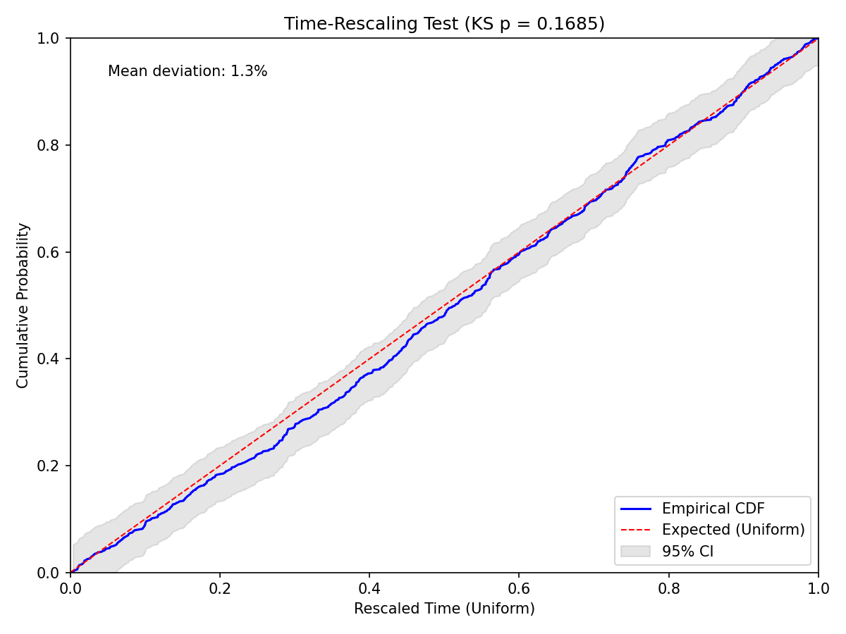
The time-rescaling test assesses whether the fitted hazard model produces inter-event intervals consistent with a Poisson process. Under the correct model, rescaled inter-event times should follow Exp(1), and their cumulative distribution should be uniform.
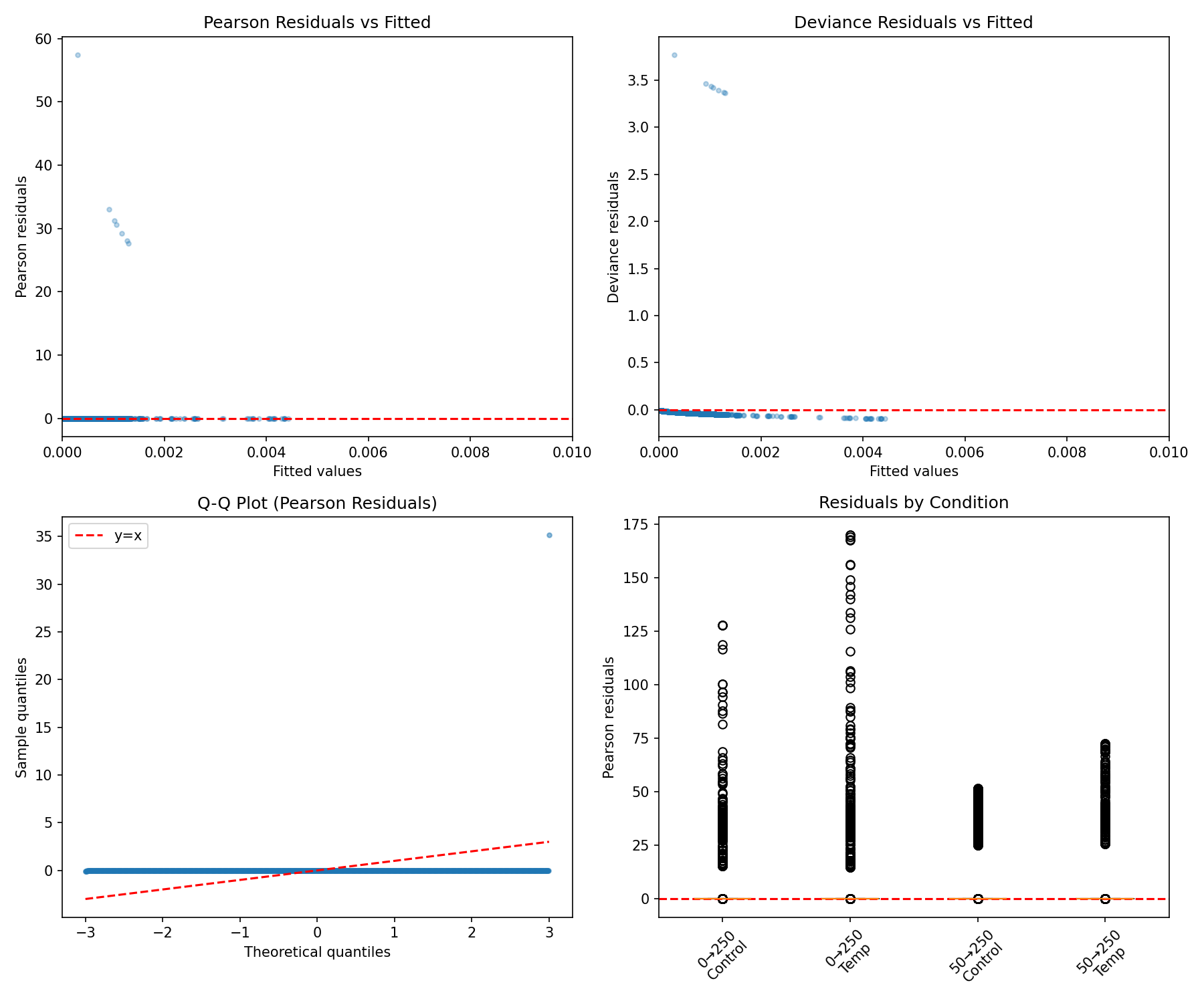
Pearson residuals: Mean = 0.0001, SD = 1.01, Skew = 40.7, Kurtosis = 2440
Large residuals: 7,288 observations (0.09%) with \(|r| > 3\)
Time-rescaling: KS statistic = 0.041, p = 0.17, mean deviation = 1.3%
The high skewness and kurtosis of residuals reflect the zero-inflated nature of event data (most frames have no events). The time-rescaling test passes at conventional significance levels, supporting the adequacy of the hazard model specification.
Bootstrap resampling (100 track-level resamples) was used to estimate 95% confidence intervals for all kernel parameters.
| Parameter | Estimate | 95% CI | Interpretation |
|---|---|---|---|
| \(A\) (fast amplitude) | 0.456 | [0.409, 0.499] | Excitatory component weight |
| \(\alpha_1\) (fast shape) | 2.22 | [1.93, 2.65] | \(\sim\)2 processing stages |
| \(\beta_1\) (fast scale, s) | 0.132 | [0.102, 0.168] | Stage time constant |
| \(B\) (slow amplitude) | 12.54 | [12.43, 12.66] | Suppressive component weight |
| \(\alpha_2\) (slow shape) | 4.38 | [4.30, 4.46] | \(\sim\)4 processing stages |
| \(\beta_2\) (slow scale, s) | 0.869 | [0.852, 0.890] | Stage time constant |
| Derived timescales | |||
| \(\tau_1\) (fast mean, s) | 0.294 | [0.268, 0.326] | Fast component timescale |
| \(\tau_2\) (slow mean, s) | 3.81 | [3.79, 3.84] | Slow component timescale |
| Peak fast (s) | 0.162 | [0.147, 0.181] | Time of fast peak |
| Peak slow (s) | 2.94 | [2.93, 2.96] | Time of slow peak |
Turn angle and duration distributions from 319 filtered events (turn duration \(> 0.1\) s) were used to parameterize trajectory simulation.
| Metric | Value | 95% Range | Best-Fit Distribution |
|---|---|---|---|
| Turn Angle | |||
| Mean | \(6.8^\circ\) | Normal(\(\mu = 6.8^\circ\), \(\sigma = 86.2^\circ\)) | |
| SD | \(86.2^\circ\) | ||
| Absolute mean | \(68.6^\circ\) | ||
| Turn Duration | |||
| Mean | 1.55 s | Lognormal(\(s = 0.59\), scale \(= 1.29\) s) | |
| Median | 1.10 s | [0.30, 6.85] s | |
| SD | 1.06 s | ||
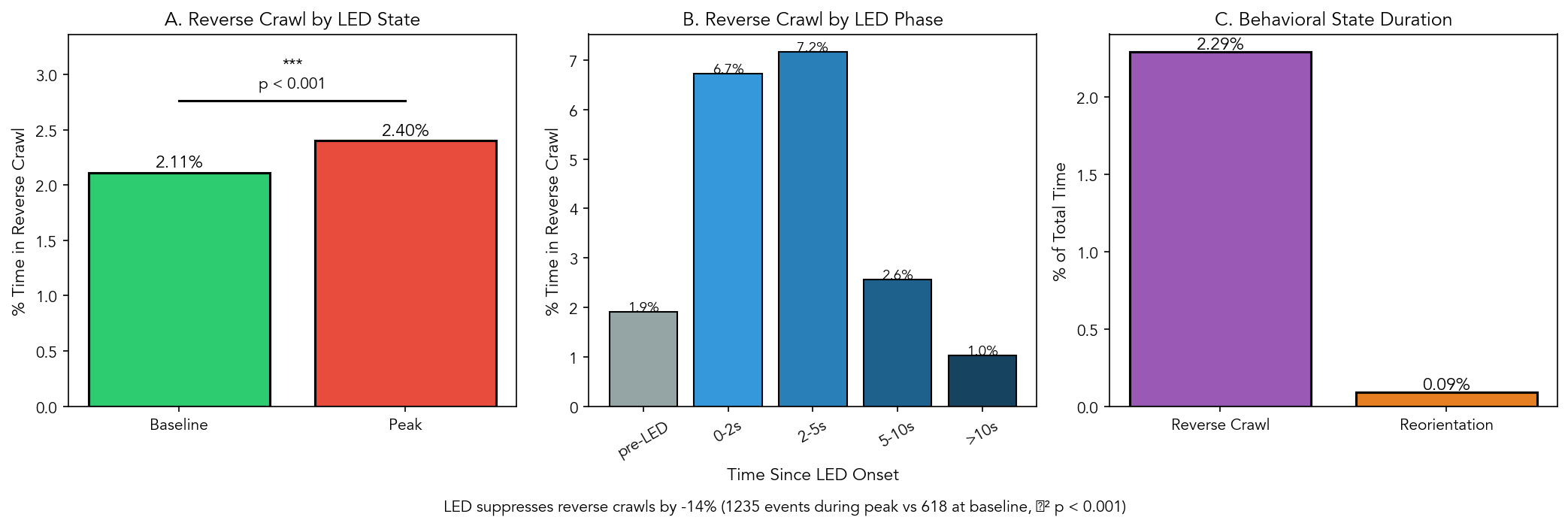
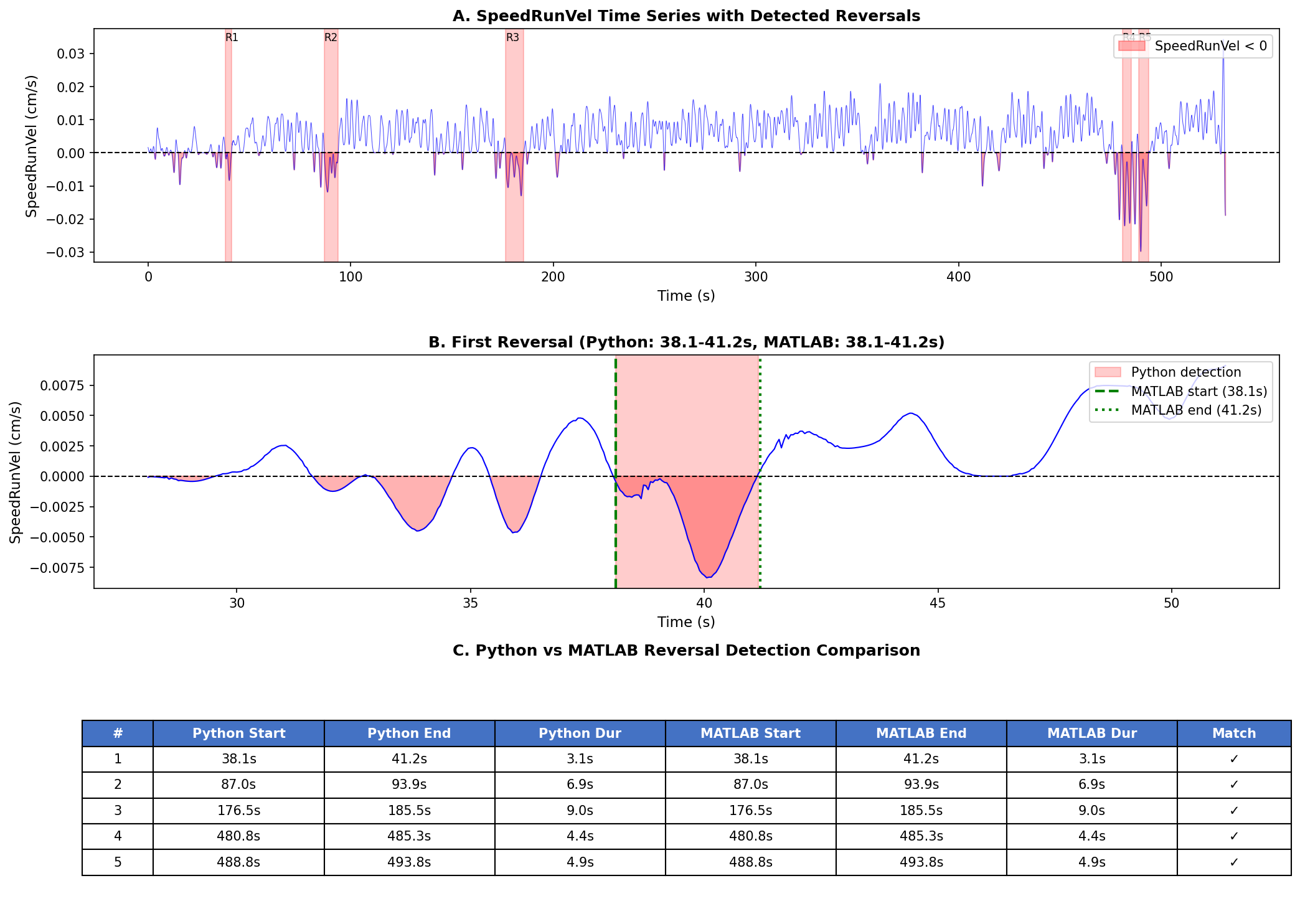
Reverse crawl detection using Mason Klein’s algorithm (SpeedRunVel \(< 0\) for \(\geq 3\) s) identified 1,853 reversal events across all 14 experiments. In contrast to reorientations (which are suppressed by LED), reverse crawls are increased during LED stimulation.
Reverse crawl detection was validated against the original MATLAB code (mason_analysis.m) on Track 2 of the reference experiment.
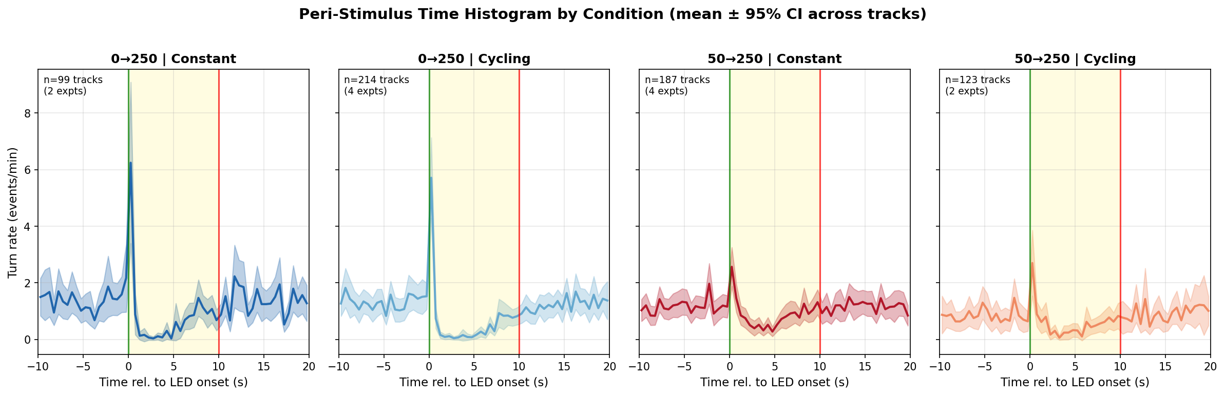
The peri-stimulus time histogram (PSTH) provides a visual comparison of model predictions against empirical event rates aligned to LED onset.
The gamma-difference kernel was fit separately to each of the four experimental conditions in the \(2\times2\) factorial design. Bootstrap confidence intervals (95%) were computed from 200 resamples.
| Condition | \(\tau_1\) (s) | 95% CI | \(\tau_2\) (s) | 95% CI | \(R^2\) | |
|---|---|---|---|---|---|---|
| 0-to-250 Constant | 0.32 | [0.23, 1.01] | 3.73 | [3.02, 4.08] | 0.94 | |
| 0-to-250 Cycling | 0.26 | [0.23, 0.71] | 4.20 | [3.79, 4.51] | 0.96 | |
| 50-to-250 Constant | 1.18 | [0.69, 2.21] | 4.53 | [3.64, 5.44] | 0.95 | |
| 50-to-250 Cycling | 0.44 | [0.23, 0.87] | 4.50 | [3.69, 5.19] | 0.81 |
Key finding: The 50-to-250 Constant condition shows a 4-fold slower fast timescale (\(\tau_1 = 1.18\) s vs \({\sim}0.3\) s), suggesting that baseline neural excitation modulates sensory transduction speed.
| Model | Parameters | \(R^2\) | AIC | Interpretation |
|---|---|---|---|---|
| Raised Cosine (12 basis) | 12 | 0.974 | \(-3386\) | Overparameterized |
| Gamma-Difference | 6 | 0.968 | \(-357\) | Biologically interpretable |
| Alpha-Difference | 4 | 0.950 | 108 | Intermediate |
| Double Exponential | 4 | 0.811 | 1432 | No shape control |
| Single Exponential | 2 | \(<0\) | 1007 | Too simple |
The gamma-difference model achieves near-optimal fit quality (\(R^2 = 0.968\)) with half the parameters of the raised-cosine basis, while providing biological interpretability (timescales map to neural processes).
Note: The single exponential model shows \(R^2 < 0\) because it cannot capture the biphasic (suppression-then-recovery) kernel shape. A negative \(R^2\) indicates the model performs worse than predicting the mean, which is expected when fitting a monotonic decay to a non-monotonic target.
Event durations from Mason Klein run tables and trajectory segmentation characterize the temporal structure of larval behavior across conditions.
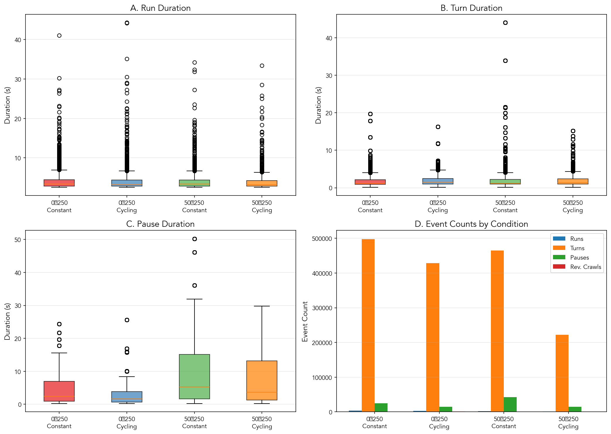
runT); no significant condition
effect (Kruskal-Wallis \(p = 0.08\)).
(B) Turn durations show significant condition effects
(\(p < 0.001\)).
(C) Pause durations vary significantly across
conditions (\(p < 0.001\)), with
50-to-250 conditions showing longer pauses. (D) Event
counts by condition and type. These distributions may inform future
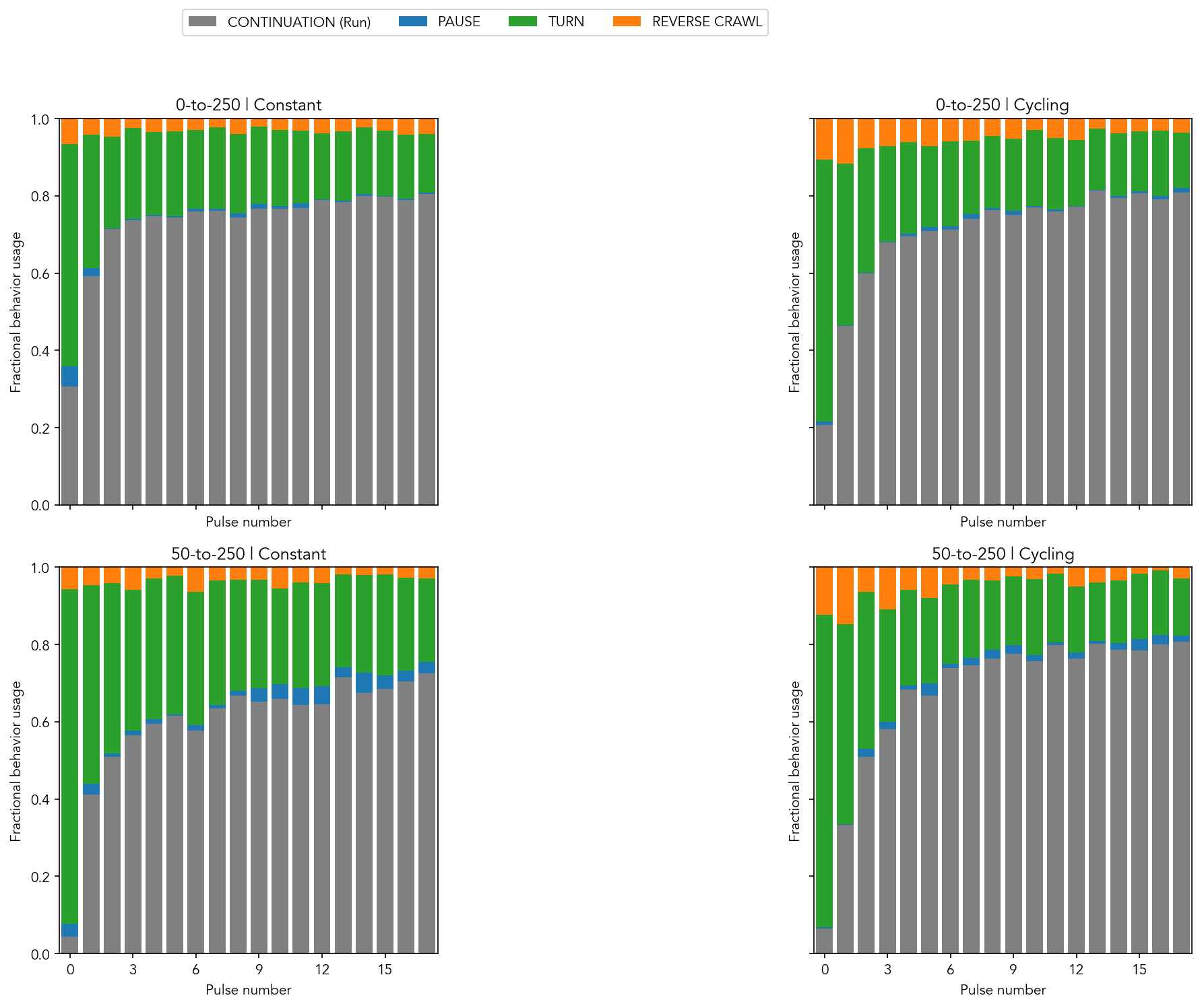
phenotype identification.Behavioral state fractions (run, pause, turn, reverse crawl) were computed for each pulse across the 20-minute experiments. The stacked bar plots reveal systematic shifts in behavioral allocation over successive pulses.